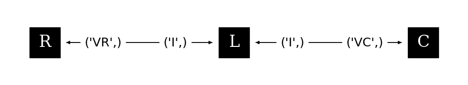
Series RLC Circuit

Such a circuit is defined by the following equations:

\[\begin{split}\begin{align} \text{R}&: V_R = I_R R \\ \text{L}&: V_L = L\frac{dI_L}{dt} \\ \text{C}&: I_C = C\frac{dV_C}{dt} \end{align}\end{split}\]

Additionally, there are the Kirchhoff equations:

\[\begin{split}I_R = I_L = I_C \equiv I \\ V_R + V_L + V_C = 0\end{split}\]

These equations may be written more succintly as

\[\begin{split}\begin{align} \text{R}&: V_R = IR \\ \text{L}&: \frac{dI}{dt} = - (V_R + V_C) / L \\ \text{C}&: \frac{dV_C}{dt} = I / C \end{align}\end{split}\]

Then the needed variables are clear: (VR, I, VC), Where 2 equations are differential and 1 is algebraic

import matplotlib.pyplot as plt
import numpy as np
from matplotlib import rc

rc("font", family="serif", size=15)
rc("savefig", dpi=600)
rc("figure", figsize=(8, 6))
rc("mathtext", fontset="dejavuserif")
rc("lines", linewidth=3)
from networkx import DiGraph

from stream import Aggregator, Calculation, unpacked

class R(Calculation):
    def __init__(self, R):
        self.R = R
        self.name = "R"

    @unpacked
    def calculate(self, VR, *, I):
        return VR - I * self.R

    @property
    def mass_vector(self):
        return (False,)

    @property
    def variables(self):
        return {"VR": 0}

class L(Calculation):
    def __init__(self, L):
        self.L = L
        self.name = "L"

    @unpacked
    def calculate(self, I, *, VR, VC):
        return -(VR + VC) / self.L

    @property
    def mass_vector(self):
        return (True,)

    @property
    def variables(self):
        return {"I": 0}

class C(Calculation):
    def __init__(self, C):
        self.C = C
        self.name = "C"

    @unpacked
    def calculate(self, VC, *, I):
        return I / self.C

    @property
    def mass_vector(self):
        return (True,)

    @property
    def variables(self):
        return {"VC": 0}

r, l, c = R(1.0), L(1.0), C(1.0)

g = DiGraph()
g.add_edge(r, l, variables=("VR",))
g.add_edge(c, l, variables=("VC",))
g.add_edge(l, r, variables=("I",))
g.add_edge(l, c, variables=("I",))

agr = Aggregator(g)

plt.figure(figsize=(12, 2))
agr.draw(
    node_options=dict(pos={r: (0, 0), l: (1, 0), c: (2, 0)}, node_size=2000, font_size=24),
    edge_options=dict(label_pos=0.3, font_size=18),
)
plt.box()

from stream.analysis.report import report

report(agr)

Contains 3 Equations, 3 Nodes, 4 Edges.

Calculation	Type	Equation No.	Unset	Set Externally	Missing
R	R	0 - 1
L	L	1 - 2
C	C	2 - 3

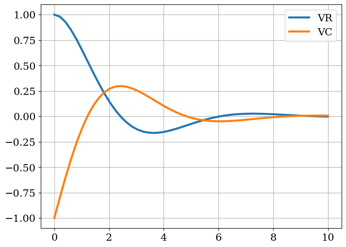
y0 = np.array([1, 1.0, -1])
time = np.linspace(0, 10)

sol = agr.solve(y0=y0, time=time, yp0=agr.compute(y0, 0))

plt.figure(figsize=(8, 6))
plt.plot(time, sol[:, 0], label="VR")
plt.plot(time, sol[:, 2], label="VC")
plt.legend()
plt.grid()
plt.show()