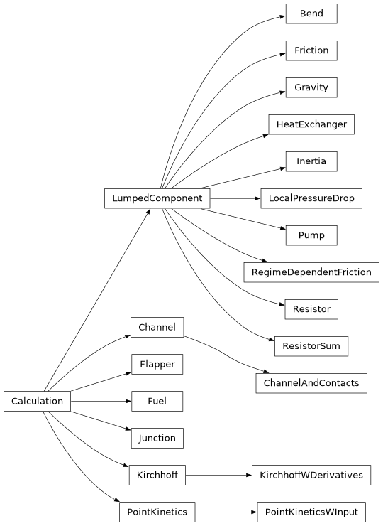
Calculations

Includes several predefined thermohydraulic calculations. These calculations are derived from Calculation.

Currently, included here are mostly calculations regarding the incompressible 1D coolant flow scheme. Other notable members are Fuel, the heat diffusion descriptor, and PointKinetics, the point-reactor neutronics descriptor.

Summary of Available Calculations

Channel	A channel in a reactor core, this model utilizes the incompressible flow assumption.
ChannelAndContacts	This class assumes two walls encompass a channel.
Flapper	A Flapper has 2 states, open or close.
Friction	Resistor quadratic in flow using a given friction coefficient
Fuel	Represents a solid component in which heat is generated and/or transferred.
Gravity	A Calculation describing in a 0D manner the pressure difference incurred by gravity, i.e. \(\Delta p = \rho g \Delta h\).
HeatExchanger	This heat exchanger doesn't care about input temperature, it always returns the same temperature.
Inertia	Flow inertia.
Junction	A junction calculation should be used anywhere several hydraulic inputs and outputs meet.
Kirchhoff	Dictates flow in a given circuit for an incompressible liquid
KirchhoffWDerivatives	A Kirchhoff Calculation containing \(\ddot{m}\)
LocalPressureDrop	Local pressure drop due to expansion or contraction according to Idelchik chapter 4.
PointKinetics	The Point Kinetics model is the simplest Neutronics dynamical model.
PointKineticsWInput	The same good-old PK, but with added power_input
Pump	Hydraulic component constraining \(\Delta p\) or \(\dot{m}\).
RegimeDependentFriction	Friction resistor which depends on the Reynolds number, see regime_dependent_friction
Resistor	A simple linear resistor to flow.
ResistorSum	Adding several LumpedComponent in series, into a single calculation.
Bend	Pressure drop due to a low relative curvature bend in a smooth circular/square pipe according to Idelchik chapter 6.

Heat Diffusion

A calculation depicting heat diffusion in a solid (supposedly material or cladding).

Discretizing the Heat Equation

Calculate the temporal derivative of temperatures according to the heat equation, which is, in this case:

\[\rho c_p \frac{\partial T}{\partial t} - \nabla\cdot(k\nabla T) = q'''\]

The medium is considered 2D in both the Cartesian and the Polar case.

Cartesian Discretization:

Integrating and writing the terms, while assuming y-symmetry. Cell \((i,j)\) reads \(i\) th cell from the top and \(j\) th cell from the left.

1. Temporal derivative

   \[\int_{V_{ij}} \rho c_p\frac{\partial T}{\partial t} dV = \rho_{ij} c_{p,ij}\frac{\partial T_{ij}}{\partial t} V_{ij}\]

2. Power Source

   \[\int_{V_{ij}} q'''dV = P_{ij}\]

3. Diffusive Term

   \[\int_{V_{ij}} \nabla\cdot(k\nabla T)dV = \oint_{\partial V_{ij}}(k\nabla T)\cdot dA\]

   Cells are boxes, so in the x-direction:

   \[= \left[(k\nabla T)_{i,j+1/2} - (k\nabla T)_{i,j-1/2}\right]A_i\]

   The thermal resistance going from one cell center to the other is just

   \[r_{ij, i(j+1)} = \frac{\Delta x_{ij}}{2k_{ij}} + \frac{\Delta x_{i(j+1)}}{2k_{i(j+1)}} + 1 / h_{ij, i(j+1)}\]

   Where \(h\) is contact conductance. Then, the flux is taken as:

   \[(k\nabla T)_{i,j+1/2} = (T_{i,j+1} - T_{i,j}) / r_{ij, i(j+1)}\]

   At the boundaries, the wall temperatures are used in a similar fashion, such that the temperature gradient is taken as one-sided.

Polar Discretization:

For the polar case, azimuthal symmetry is assumed, and the temperature is a function of the radius \(r\) and height \(z\). Similar to the Cartesian case, here cell \((i,j)\) reads \(i\) th cell from the top and \(j\) th cell from the smallest radius (0 for a cylinder). The integration is the same (since the \(\nabla_\hat{r}\) and \(\nabla_\hat{z}\) components are just \(\partial_r\) and \(\partial_z\), respectively), but the volumes and cell areas are \(r\)-dependent. Specifically:

\[\begin{split}\begin{align} A_{i, j-1/2} &= 2\pi r_{j-1/2}\Delta z_i \\ A_{i-1/2, j} = A_{i+1/2, j} &= \pi (r_{j+1/2} ^ 2 - r_{j-1/2} ^ 2) \\ V_{ij} &= \pi (r_{j+1/2} ^ 2 - r_{j-1/2} ^ 2)\Delta z_i \\ \end{align}\end{split}\]

The thermal resistance is then computed in the same manner using the distances between cell centers \(\Delta r, \Delta z\).

class Fuel(z_boundaries, x_boundaries, material, y_length, power_shape, heat_func=<function x_diffusion>, T_wall_func=<function wall_temperature>, x_contacts=None, z_contacts=None, meat_indices=None, name='Fuel')

Bases: Calculation

Represents a solid component in which heat is generated and/or transferred. An internal volumetric heat source may be supplied and heat is conducted in up to two dimensions.

Geometry is introduced through 2 explicit dimensions, termed \(x\) and \(z\) and an auxiliary dimension termed \(y\) in which symmetry is assumed. Providing heat_func may allow one to support generally many continuous 2D structures. Explicitly supported geometries are:

• Rectangular (x_diffusion or xz_diffusion).

• Cylindrical (r_diffusion or rz_diffusion) - in this case the radial dimension is \(x\), and \(y\) represents an azimuthal symmetry.

See more in Discretizing the Heat Equation for the according Cartesian and Polar discretizations of the heat equation.

Boundary conditions are supplied through extraneous temperature and conductance pairs, which are termed left, right, top, and bottom, and couple to the 2D mesh \(z \times x\) accordingly. Be aware that there is an inherent difference between (left, right) and (top, bottom). While this calculation provides its calculated wall temperatures at the (left, right) walls (so that other calculations may transfer heat from it), the (top, bottom) wall temperatures are calculated but not provided.

Defaults:

• Geometry is rectangular

• Contacts are assumed infinitely conductive.

• Meat_indices describes the entire plate as meat.

• heat_func describes x-diffusion only.

• T_wall_func assumes zero-inertia at wall.

• power_shape is assumed uniform.

Parameters:

• z_boundaries (Meter) – Boundaries crossing the z-axis

• x_boundaries (Meter) – Boundaries crossing the x-axis

• material (Solid) – Bulk properties. Can be of shape: (z_cells, x_cells) matrix

• y_length (Meter) – Length of the symmetric dimension.

• power_shape (Array2D) – Shape of power distribution over the fuel meat. Should have the same shape as the fuel meat.

• heat_func (Callable) – A function computing the temporal derivative of bulk temperatures.

• T_wall_func (Callable) – A function computing wall temperatures.

• x_contacts (WPerM2K) – Contact conductivity of x_axis contacts. This means its shape should be (z_cells, x_cells + 1), i.e. including outer boundaries.

• z_contacts (WPerM2K) – Contact conductivity of z_axis contacts. This means its shape should be (z_cells + 1, x_cells), i.e. including outer boundaries.

• meat_indices (Array2D) – Meat placements, specifically where power would be deposited (at meat_indices = 1).

• name (str) – Name of the calculation.

calculate(variables, *, power, T_left=None, T_right=None, T_top=None, T_bottom=None, h_left=None, h_right=None, h_top=None, h_bottom=None)

Calculating temperatures inside fuel and at the edges. If wall temperatures are not given

Parameters:

• variables (Celsius) – Temperatures inside (and on edges) of Fuel element

• power (Watt) – Generated power at meat.

• T_left (Celsius) – Temperature just outside the left edge

• T_right (Celsius) – Temperature just outside the right edge

• T_top (Celsius) – Temperature just outside the top edge

• T_bottom (Celsius) – Temperature just outside the bottom edge

• h_left (WPerM2K) – Left wall conductance

• h_right (WPerM2K) – Right wall conductance

• h_top (WPerM2K) – Top wall conductance

• h_bottom (WPerM2K) – Bottom wall conductance

Returns:

Functional output – Temporal derivative (for inner temperatures) and error for walls

Return type:

CPerS or C

indices(variable, asking=None)

Parameters:

variable (str)

Return type:

int | slice | ndarray

load(state)

Given a state of the calculation, return the untagged corresponding array, which may be used to calculate the next step.

The default method implemented here assumes the state is completely described by the variables presented in self.variables.

Parameters:

state (CalcState) – Tagged information regarding system state

Returns:

y – Calculation ready array

Return type:

Array1D

save(vector, **_)

Parameters:

vector (Sequence[float])

Return type:

dict[str, float | ndarray]

property mass_vector: Sequence[bool]

property variables: dict[str, int | slice | ndarray]

class Solid(density, specific_heat, conductivity)

Bases: object

Simple bulk properties of a material

Parameters:

• density (KgPerM3)

• specific_heat (JPerKgK)

• conductivity (WPerMK)

classmethod from_array(array)

Create a Solid from an array of Solid scalars

Parameters:

array (np.array) – An array of Solid objects, where each instance has scalar values

Returns:

An instance with array-shaped fields.

Return type:

Solid

Examples

>>> Solid.from_array(np.array([Solid(1, 2, 3), Solid(4, 5, 6)]))
Solid(density=array([1, 4]), specific_heat=array([2, 5]), conductivity=array([3, 6]))

conductivity: float | ndarray

density: float | ndarray

specific_heat: float | ndarray

class Walls(left=None, right=None, top=None, bottom=None)

Bases: object

Simple 2D walls container

Parameters:

• left (float | ndarray)

• right (float | ndarray)

• top (float | ndarray)

• bottom (float | ndarray)

bottom: float | ndarray

left: float | ndarray

right: float | ndarray

top: float | ndarray

property x

The x (lateral) values of the walls

property z

The z (axial) values of the walls.

cylindrical_areas_volumes(r, z)

Calculate areas and cell volumes for a cylindrical mesh

Parameters:

• r (Meter) – Boundaries crossing the r-axis.

• z (Meter) – Boundaries crossing the z-axis.

Return type:

Areas and volumes for rz diffusion

Examples

>>> r = np.array([0, 1, 4, 14]); z = np.array([0, 3, 5, 15])
>>> r_areas, z_areas, volumes = cylindrical_areas_volumes(r=r, z=z)
>>> r_areas / (2 * np.pi)
array([[  0.,   3.,  12.,  42.],
       [  0.,   2.,   8.,  28.],
       [  0.,  10.,  40., 140.]])
>>> z_areas / np.pi
array([[  1.,  15., 180.],
       [  1.,  15., 180.],
       [  1.,  15., 180.],
       [  1.,  15., 180.]])
>>> volumes / np.pi
array([[   3.,   45.,  540.],
       [   2.,   30.,  360.],
       [  10.,  150., 1800.]])

r_diffusion(T, T_walls, material, power, x, z, contacts, **_)

1D heat diffusion (r) in a 2D cylindrical mesh (r, z). Assumes azimuthal symmetry.

Calculates the temporal derivative of temperatures according to the heat equation.

Parameters:

• T (Celsius) – Material temperature

• T_walls (Walls) – Wall temperatures, inner and outer radii.

• material (Solid) – a Solid object for thermal properties

• power (Watt) – Power, a source term.

• x (Meter) – Boundaries crossing the r-axis.

• z (Meter) – Boundaries crossing the z-axis.

• contacts (Sequence[WPerM2K]) – indices and transfer coefficients for Fuel-Clad contacts

Returns:

dT/dt – for the heat equation in the material. r diffusion is assumed.

Return type:

CPerS

rz_diffusion(T, T_walls, material, power, x, z, contacts, **_)

2D heat diffusion in a 2D cylindrical mesh (r, z). Assumes azimuthal symmetry.

Calculates the temporal derivative of temperatures according to the heat equation.

Parameters:

• T (Celsius) – Material temperature

• T_walls (Walls) – Wall temperatures, inner and outer radii.

• material (Solid) – a Solid object for thermal properties

• power (Watt) – Power, a source term.

• x (Meter) – Boundaries crossing the r-axis.

• z (Meter) – Boundaries crossing the z-axis.

• contacts (Sequence[WPerM2K]) – indices and transfer coefficients for Fuel-Clad contacts

Returns:

dT/dt – for the heat equation in the material. rz diffusion is assumed.

Return type:

CPerS

x_diffusion(T, T_walls, material, power, x, z, contacts, y)

1D heat diffusion (x) in a 2D mesh (x, z)

Calculates the temporal derivative of temperatures according to the heat equation.

Parameters:

• T (Celsius) – Material temperature

• T_walls (Walls) – Wall temperatures, left and right (in the case of polar coordinates, inner and outer radii)

• material (Solid) – a Solid object for thermal properties

• power (Watt) – Power, a source term.

• x (Meter) – Boundaries crossing the x-axis.

• z (Meter) – Boundaries crossing the z-axis.

• y (Meter) – In the Cartesian case, the length of the non-described (meaning symmetric) dimension.

• contacts (Sequence[WPerM2K]) – indices and transfer coefficients for Fuel-Clad contacts

Returns:

dT/dt – for the heat equation in the material. Only x-diffusion is assumed.

Return type:

CPerS

xz_diffusion(T, T_walls, material, power, x, z, contacts, y)

2D heat diffusion in a 2D mesh (x, z)

Calculates the temporal derivative of temperatures according to the heat equation.

Parameters:

• T (Celsius) – Material temperature

• T_walls (Walls) – Wall temperatures, left and right (in the case of polar coordinates, inner and outer radii)

• material (Solid) – a Solid object for thermal properties

• power (Watt) – Power, a source term.

• x (Meter) – Boundaries crossing the x-axis.

• z (Meter) – Boundaries crossing the z-axis.

• y (Meter) – In the Cartesian case, the length of the non-described (meaning symmetric) dimension.

• contacts (Sequence[WPerM2K]) – indices and transfer coefficients for Fuel-Clad contacts

Returns:

dT/dt – for the heat equation in the material. xz-diffusion is assumed.

Return type:

CPerS

See also

x_diffusion

Point Kinetics

A calculation for the point kinetics neutronics model

class InputReactivity(*args, **kwargs)

Bases: Protocol

class OneWayToSCRAM(*values)

Bases: StrEnum

NORMAL = 'NORMAL'

SCRAM = 'SCRAM'

class PointKinetics(generation_time, delayed_neutron_fractions, delayed_groups_decay_rates, temp_worth=None, ref_temp=None, controls=None, name='PK')

Bases: Calculation

The Point Kinetics model is the simplest Neutronics dynamical model. It assumes spatial and spectral flux shapes are either unimportant or fixed, and deals with the flux by a single number which may be thought of as the population size or power. The delayed neutron yield processes are paramount to the dynamical description, thus they are characterized as well, bundled into k characteristic groups. The equations are:

\[\begin{split}\dot{P} &= \frac{\rho - \beta}{\Lambda} P + \sum_k C_k\lambda_k + \frac{S}{\Lambda} \\ \dot{C}_k &= - C_k\lambda_k + \frac{\beta_k}{ \Lambda} P\end{split}\]

Where:

• \(P\): power

• \(\rho\): reactivity

• \(\beta\): total delayed neutron fraction (1$)

• \(\Lambda\): generation time

• \(C_k\): k-group’s contribution to power

• \(\lambda_k\) : k-group’s decay rate.

• \(S\): Power Source

In this particular calculation, the reactivity may be influenced by a linear thermal feedback \(\rho = \rho_0 + \alpha_c T_c + \alpha_f T_f\) by corresponding coolant and fuel elements.

Parameters:

• generation_time (Second) – mean time between neutron generations.

• delayed_neutron_fractions (Array1D) – the fractional yield of neutrons in defined delay groups. 1$ worth is the total.

• delayed_groups_decay_rates (PerS) – each group’s decay rate.

• temp_worth (dict[Calculation, PerC] or None) – a dictionary whose keys are fuel or channel elements, and values are their temperature worth.

• ref_temp (dict[Calculation, Celsius] or None) – At such temperature/s, temperature feedback is 0.

• controls (ReactivityController) – Induces reactivity due to a state-machine model of the reactor controls, including any postulated accidents. By default, does nothing.

• name (str)

calculate(variables, *, T=None, source=None, t, **kwargs)

Calculate \(\frac{d}{dt}(P, \vec{C}_k)\)

Parameters:

• variables (Sequence[float]) – \((P, \vec{C}_k)\)

• source (dict[Calculation, Watt] or None) – External Power Sources

• T (dict[Calculation, Celsius] or None) – Temperatures which affect reactivity through ‘temp_worth’

• t (Second or None) – Time, used to call input_reactivity

Returns:

dPdt – the change in power and the delayed power fractions

Return type:

Array1D

change_state(variables, *, t, **kwargs)

Parameters:

• variables (Sequence[float])

• t (float | ndarray)

reactivity(T, input_reactivity)

Calculate the reactivity, given temperature feedback

Parameters:

• T (dict[Calculation, Array1D]) – Mapping of Calculation to temperatures (say in channels, fuels)

• input_reactivity (float)

Returns:

rho – Calculated reactivity

Return type:

float

save(vector, *, T=None, source=None, t, **kwargs)

Given input for “calculate” (which is a legal state of the system), tag the information, i.e. create a “State” and return it.

Parameters:

• vector (Sequence[float])

• source (dict[Calculation, Watt]) – External Power Sources

• T (dict[Calculation, Celsius]) – Temperatures which affect reactivity through ‘temp_worth’

• t (Second or None) – Time, used to call input_reactivity

Returns:

state – Tagged information regarding system state

Return type:

CalcState

should_continue(variables, *, t, **kwargs)

Parameters:

• variables (Sequence[float])

• t (float | ndarray)

Return type:

bool

property mass_vector: Sequence[bool]

property variables: dict[str, int | slice | ndarray]

class PointKineticsWInput(generation_time, delayed_neutron_fractions, delayed_groups_decay_rates, temp_worth=None, ref_temp=None, controls=None, name='PK')

Bases: PointKinetics

The same good-old PK, but with added power_input

An additional distinction is made between power (=total power) and pk_power. Such a distinction is important when regarding additional sources of power, stemming from the decay of fission products, activated structure materials, gamma absorption and more. These sources should be passed to this model through power_input.

See also

decay_heat

Parameters:

• generation_time (Second) – mean time between neutron generations.

• delayed_neutron_fractions (Array1D) – the fractional yield of neutrons in defined delay groups. 1$ worth is the total.

• delayed_groups_decay_rates (PerS) – each group’s decay rate.

• temp_worth (dict[Calculation, PerC] or None) – a dictionary whose keys are fuel or channel elements, and values are their temperature worth.

• ref_temp (dict[Calculation, Celsius] or None) – At such temperature/s, temperature feedback is 0.

• controls (ReactivityController) – Induces reactivity due to a state-machine model of the reactor controls, including any postulated accidents. By default, does nothing.

• name (str)

calculate(variables, *, T=None, source=None, t, power_input=None, **kwargs)

Parameters:

• variables (Sequence[float])

• T (dict[Calculation, float | ndarray])

• source (float | ndarray | None)

• t (float | ndarray)

• power_input (float | ndarray | None)

Return type:

ndarray

property mass_vector: Sequence[bool]

property variables: dict[str, int | slice | ndarray]

class ReactivityController(input_reactivity=None, state_machine=<function just.<locals>._val>, initial_state=OneWayToSCRAM.NORMAL, initial_time=0.0, abort_states=None)

Bases: object

Input to PointKinetics which depicts the reactivity worth inserted due to the reactor control system or postulated events. The control system is modelled as a StateMachine. This system can include the Reactor Protection System (RPS), Reactor Control and Monitoring System (RCMS) and such.

The state machine is completely user defined such through an ‘Enum’ class. Then, two functionalities are requited: 1. The reactivity worth response of the controller \(w_c(s, t_s, t)\) where \(s\) the current state, \(t_s\) the time in which this state was invoked, and \(t\) the current time. 2. The state machine transfer function \(p: s \rightarrow s'\) where p receives \(p(s, t, P, \dot{P}, ...)\) provided by PointKinetics during simulation.

After simulation, the log attribute of this class contains the history of states, which can be used for analysis and plotting.

Parameters:

• input_reactivity (InputReactivity or None) – The reactivity worth response of the controller \(w_c(s, t_s, t)\) where \(s\) the current state, \(t_s\) the time in which this state was invoked, and \(t\) the current time. If None, then no reactivity is inserted.

• state_machine (StateMachine) – The state machine transfer function \(p: s \rightarrow s'\) where p receives \(p(s, t, P, \dot{P}, ...)\) provided by PointKinetics during simulation. If None, then the state machine is static and does not change state.

• initial_state (Enum) – Initial state

• initial_time (Second) – Initial time

• abort_states (set[Enum] or None) – States for which the simulation should stop, through the should_continue function.

change_state(t, power, dPdt, **kwargs)

Parameters:

• t (float | ndarray)

• power (float | ndarray)

• dPdt (float | ndarray)

Return type:

S

reset()

should_continue(t)

Parameters:

t (float | ndarray)

Return type:

bool

worth(t)

Reactivity worth inserted by the controller as function of time

Parameters:

t (float | ndarray)

Return type:

float

worth_history(t)

Parameters:

t (float | ndarray)

Return type:

float

class StateMachine(*args, **kwargs)

Bases: Protocol

Reactor control state machine. Assued Markovian

SCRAM_at_power(power_limit='__no__default__', power='__no__default__', **kwargs)

Parameters:

• power_limit (float | ndarray)

• power (float | ndarray)

temperature_reactivity(T, T0, weights)

Calculate the reactivity, given temperature feedback

\[\rho = - \sum_i \vec{w}_i \cdot (\vec{T}-\vec{T}_0)_i\]

Parameters:

• T (dict[Calculation, Array]) – Mapping of Channel calculation to temperatures in channel

• T0 (dict[Calculation, Array]) – Reference Temperatures

• weights (dict[Calculation, Array])

Returns:

rho – Calculated reactivity

Return type:

float

Channel

Defines both coolant properties and data, and the temporal coolant temperature derivative calculation.

class Channel(z_boundaries, fluid, pipe, pressure_func=<function pressure_diff>, name='Channel')

Bases: Calculation

A channel in a reactor core, this model utilizes the incompressible flow assumption. The Channel is considered 1D so that there is no attention to transverse flow.

Parameters:

• z_boundaries (Meter) – boundaries (no. cells + 1). Must be strictly monotonous.

• fluid (LiquidFuncs) – Coolant properties, see light_water or heavy_water.

• pipe (EffectivePipe) – Channel geometry

• pressure_func (Callable) – A function determining the pressure gradient in the channel.

• name (str)

calculate(variables, *, T_left=None, T_right=None, h_left=0.0, h_right=0.0, Tin, Tin_minus=None, mdot, mdot2=None, **kwargs)

Calculate rate of temperature change in each cell by means of First Order Upwind and pressure difference error.

Parameters:

• variables (Sequence[float]) – Input variables, see Channel.variables

• T_left (Celsius) – Left and right boundary (wall) temperatures

• T_right (Celsius) – Left and right boundary (wall) temperatures

• h_left (WPerM2K) – Left and right heat transfer coefficients

• h_right (WPerM2K) – Left and right heat transfer coefficients

• Tin (Celsius) – Inlet boundary temperature

• Tin_minus (Celsius) – Outlet boundary temperature

• mdot (KgPerS) – Mass flow rate

• mdot2 (KgPerS2) – \(\ddot{m}\), time derivative of mdot

Returns:

F(y, t) – Which comprises the rate of temperature change and a pressure difference constraint.

Return type:

Array1D

indices(variable, asking=None)

Parameters:

variable (str)

Return type:

int | slice | ndarray

save(vector, *, T_left=None, T_right=None, Tin, Tin_minus=None, mdot, p_abs=None, mdot2=None, **kwargs)

Given input for “calculate” (which is a legal state of the system), tag the information, i.e. create a “State” and return it.

Parameters:

• vector (Sequence[float]) – Input variables, see Channel.variables

• T_left (Celsius) – Left and right boundary (wall) temperatures

• T_right (Celsius) – Left and right boundary (wall) temperatures

• Tin (Celsius) – Inlet boundary temperature

• Tin_minus (Celsius) – Outlet boundary temperature

• mdot (KgPerS) – Mass flow rate

• p_abs (Pascal or None) – Pressure at the channel inlet. If given, the state will include the absolute pressure at each cell

• mdot2 (KgPerS2) – \(\ddot{m}\), time derivative of mdot

Returns:

state – The physical state of the channel, which includes additionally absolute_pressure and the Re number in each cell.

Return type:

CalcState

property mass_vector: Sequence[bool]

property variables: dict[str, int | slice | ndarray]

Mapping T_cool, pressure to vector places

class ChannelAndContacts(z_boundaries, fluid, pipe, h_wall_func=<function wall_heat_transfer_coeff>, pressure_func=<function pressure_diff>, name='CC')

Bases: Channel

This class assumes two walls encompass a channel. It calculates the heat transfer coefficient to each wall in addition to the Channel properties.

Parameters:

• z_boundaries (Meter) – boundaries (no. cells + 1). Must be strictly monotonous.

• fluid (LiquidFuncs) – Coolant properties

• pipe (EffectivePipe) – Channel geometry

• h_wall_func (Callable) – A function determining the heat transfer coefficient

• pressure_func (Callable) – A function determining the pressure gradient in the channel.

• name (str)

See also

wall_heat_transfer_coeff, pressure_diff

calculate(variables, *, T_left=None, T_right=None, Tin, Tin_minus=None, mdot, p_abs, mdot2=None)

Parameters:

• variables (Sequence[float]) – Input variables, see ChannelAndContacts.variables

• T_left (Celsius) – Left and right boundary (wall) temperatures

• T_right (Celsius) – Left and right boundary (wall) temperatures

• Tin (Celsius) – Inlet boundary temperature

• Tin_minus (Celsius) – Outlet boundary temperature

• mdot (KgPerS) – Mass flow rate

• p_abs (Pascal) – The absolute pressure at the inlet.

• mdot2 (KgPerS2) – \(\ddot{m}\), time derivative of mdot

Returns:

F(y, t) – Which consists of the rate of temperature change, and pressure difference and wall heat transfer coefficients constraint.

Return type:

Array1D

dist_from_edge(mdot)

Computes the center distances from the channel entrance depending on flow direction.

Parameters:

mdot (KgPerS) – Mass flow rate. Sign determines flow direction.

Return type:

float | ndarray

h_wall(T_cool, T_wall, mdot, pressure, **_)

Parameters:

• T_cool (float | ndarray)

• T_wall (float | ndarray)

• mdot (float | ndarray)

• pressure (float | ndarray)

Return type:

float | ndarray | None

indices(variable, asking=None)

Parameters:

variable (str)

Return type:

int | slice | ndarray

save(vector, *, T_left=None, T_right=None, Tin, Tin_minus=None, mdot, p_abs=None, **kwargs)

Given input for “calculate” (which is a legal state of the system), tag the information, i.e. create a “State” and return it.

Parameters:

• vector (Sequence[float]) – Input variables, see ChannelAndContacts.variables

• T_left (Celsius) – Left and right boundary (wall) temperatures

• T_right (Celsius) – Left and right boundary (wall) temperatures

• Tin (Celsius) – Inlet boundary temperature

• Tin_minus (Celsius) – Outlet boundary temperature

• mdot (KgPerS) – Mass flow rate

• p_abs (Pascal or None) – Pressure at the channel inlet. If given, the state will include the absolute pressure at each cell

Returns:

state – The physical state of the channel, which includes additionally things like absolute_pressure, Re, ONB, left, ONB, right safety factor (for each wall, see BR_ONB) number in each cell.

Return type:

CalcState

property mass_vector: Sequence[bool]

property variables: dict[str, int | slice | ndarray]

Mapping T_cool, h_left, h_right, pressure to vector places

class ChannelHeatFlux(z_boundaries, fluid, pipe, pressure_func=<function pressure_diff>, name='Channel')

Bases: Channel

A channel in a reactor core. This model utilizes the incompressible flow assumption. The Channel is considered 1D so that there is no attention to transverse flow. This class differs from the Channel class by having a different way to couple with an adjunct heat producer. The Channel class gives the heat producer a heat transfer coefficient and receives its temperature, but this object is coupled by getting the heat flux itself from that neighbor.

This object is simpler, and thus less useful for actual systems, but more useful for toy problems.

Parameters:

• z_boundaries (Meter) – boundaries (no. cells + 1). Must be strictly monotonous.

• fluid (LiquidFuncs) – Coolant properties, see light_water or heavy_water.

• pipe (EffectivePipe) – Channel geometry

• pressure_func (Callable) – A function determining the pressure gradient in the channel.

• name (str)

classmethod from_channel(channel)

Make a heat flux based channel from a regular one.

Parameters:

channel (Channel)

Return type:

ChannelHeatFlux

calculate(variables, *, Tin=None, Tin_minus=None, T_left=None, T_right=None, mdot, mdot2=None, q_left=0.0, q_right=0.0)

Parameters:

• variables (Sequence[float])

• Tin (float | ndarray)

• Tin_minus (float | ndarray)

• T_left (float | ndarray)

• T_right (float | ndarray)

• mdot (float | ndarray)

• mdot2 (float | ndarray)

• q_left (float | ndarray)

• q_right (float | ndarray)

Return type:

ndarray

save(vector, q_left, q_right, **kwargs)

Parameters:

• vector (Sequence[float])

• q_left (float | ndarray)

• q_right (float | ndarray)

Return type:

dict[str, float | ndarray]

class ChannelVar(*values)

Bases: StrEnum

Enum for variable names saved in Channel calculations.

This class is useful for discoverability, and to increase coherency across the setup and analysis of channels, which are often analyzed thoroughly.

classmethod get(key, direction)

Get the variable name in a case where direction may be involved.

Parameters:

• key (str) – Variable name in general

• direction (left or right) – The directionality, in a case where the channel has multiples of the same thing.

Return type:

The appropriate enum member.

absolute_pressure = 'absolute_pressure'

gr_left = 'Gr, left'

gr_right = 'Gr, right'

h_left = 'h_left'

h_right = 'h_right'

heatflux_left = 'q, left'

heatflux_right = 'q, right'

mass_flow = 'mass_flow'

pe = 'Pe'

power = 'power'

pressure_drop = 'pressure'

re = 'Re'

static_pressure = 'static_pressure'

tbulk = 'T_cool'

tin = 'T_in'

tout = 'T_out'

twall_left = 'T_wall, left'

twall_right = 'T_wall, right'

velocity = 'velocity'

class Direction(*values)

Bases: StrEnum

Directions that are supported by the code.

We use this enum rather than literal strings because we want other places in the code to refer to these values in a way where things won’t break if we rename directions.

It is also somewhat more discoverable.

inner = 'left'

left = 'left'

outer = 'right'

right = 'right'

coolant_first_order_upwind_dTdt(T, Tin, mdot, q_left, q_right, fluid, pipe, dz)

Calculates the first order upwind differencing temperature convection equation’s temporal derivative. Essentially, this is the equation:

\[mc_p\dot{T_i} = \frac{1}{2}\dot{m}(c_{p,i}+c_{p,i-1})(T_{i-1}-T_{i}) + h\Pi (T_{wall,i} - T_i)\]

Parameters:

• T (Celsius) – Bulk temperature (assumed 1D)

• Tin (Celsius) – Inlet bulk temperature (assumed float)

• q_left (WPerM2K) – Wall heat flux

• q_right (WPerM2K) – Wall heat flux

• mdot (KgPerS) – Mass flow of coolant, assumed constant along channel

• fluid (LiquidFuncs) – Temperature and pressure dependent coolant properties

• pipe (EffectivePipe) – Geometrical properties of the channel

• dz (Meter) – Cell sizes, which may vary.

Returns:

dT/dt – the temporal derivative of the bulk temperature

Return type:

CPerS

LumpedComponent

The LumpedComponent is used as a base class for methods and properties which many other Calculations use. The overarching concept is that of a Lumped object in an idealized Kirchoff model for flow, with an analogy to electronic circuits. Most Primary Circuit Calculations just deal with changes in pressure and outlet temperature, and these often share much of their implementation. Some calculations may benefit from methods or properties of the LumpedComponent, and if they are not just LumpedComponents, they should use composition rather than inheritance, as done in Flapper.

If you want to represent a 0-dimensional, no inner-working Calculation, which only serves to have a pressure drop or a temperature change, you may find this namespace to be useful.

class LumpedComponent(*args, **kwargs)

Bases: Calculation

0-dimensional Kirchhoff-oriented flow components

An ideal simple component would only need two variables:

1. Incoming temperature (Tin)

2. Incoming mass current (mdot)

These calculations compute only the outlet temperature and the pressure difference on them. The equations are assumed to be algebraic.

T_out(*, Tin, **_)

Outlet temperature calculation.

Parameters:

Tin (Celsius) – Inlet Temperature

Return type:

float | ndarray

calculate(variables, *, mdot, Tin, Tin_minus=None, **kwargs)

Compute the algebraic residual values for this Calculation.

Parameters:

• variables (Sequence[float]) – Input variables, specifically [Tin, dp]

• Tin (Celsius) – Inlet Temperature.

• Tin_minus (Celsius or None) – Inlet Temperature in case the flow is reversed.

• mdot (KgPerS) – Mass flow rate.

• kwargs (dict) – Other input. It takes precedence over the following dict(dp=dp, Tin=Tin, mdot=mdot) when merged, which is then input for self.T_out and self.dp_out.

Returns:

errors – The error in variables

Return type:

Array1D

dp_out(*, mdot, Tin, **_)

Pressure drop calculation.

Parameters:

• mdot (KgPerS) – Mass flow rate

• Tin (Celsius) – Inlet temperature.

Return type:

Pascal

indices(variable, asking=None)

For a given variable name, return the appropriate positions in the vector

Parameters:

• variable (Name) – Name of requested variable

• asking (Calculation or None) – What calculation is asking for the indices? For example, this is important in Kirchhoff.

Returns:

indices – The place in which the calculation uses the variable, or a dictionary with variable names related to this name and their places.

Return type:

Place or dict[Calculation, Place]

property mass_vector: tuple[bool, bool]

A mass vector, which is just two False values.

property variables: dict[str, int | slice | ndarray]

All variables owned by calculation

Pumps

class Pump(pressure=None, mdot0=None, name='Pump')

Bases: LumpedComponent

Hydraulic component constraining \(\Delta p\) or \(\dot{m}\). It does not affect temperature values, merely propagates it.

If the chosen constraint is mass flow rate (\(\dot{m}=\dot{m}_0\)), then the pressure difference cannot be constrained, and vice versa. One can provide externally a time-dependent value of pressure difference or mass flow rate.

Parameters:

• pressure (Pascal or None) – Optional Static desired \(\Delta p\)

• mdot0 (KgPerS or None) – Optional Static desired \(\dot{m}\)

• name (str or None) – Optional name, see Calculation

Raises:

ValueError – If both pressure and mdot0 are not None.

calculate(variables, *, mdot, Tin, Tin_minus=None, pressure=None, mdot0=None, **_)

Parameters:

• variables (Sequence[float])

• mdot (float | ndarray)

• Tin (float | ndarray)

• Tin_minus (float | ndarray | None)

• pressure (float | ndarray | None)

• mdot0 (float | ndarray | None)

Return type:

ndarray

Resistors

Calculations that only drop the pressure when fluid flows through them.

Their electrical analogs are resistors in an electric circuit, even though most of the resistors here do not follow an Ohm’s law (i.e. they are not linear).

class Bend(fluid, hydraulic_diameter, area, bend_radius, bend_angle, friction_func=CPUDispatcher(<function turbulent_friction>), name='Bend')

Bases: LumpedComponent

Pressure drop due to a low relative curvature bend in a smooth circular/square pipe according to Idelchik chapter 6.

The appropriate diagram is 6.1, on page 424.

Parameters:

• fluid (LiquidFuncs) – Coolant properties

• hydraulic_diameter (Meter) – Hydraulic diameter of the pipe.

• area (Meter2) – Cross-sectional area of the pipe.

• bend_radius (Meter) – The pipe’s axis radius of curvature, measured from the bend center to the center of the pipe.

• bend_angle (Radians) – The pipe’s bend angle.

• friction_func (Callable[[float], float]) – Re-dependent Darcy friction function. Default is turbulent_friction.

• name (str)

dp_out(*, mdot, Tin, **_)

Parameters:

• mdot (float | ndarray)

• Tin (float | ndarray)

Return type:

float | ndarray

class DPCalculation(*args, **kwargs)

Bases: Calculation, Protocol

A calculation that has a dp_out method

dp_out(*, mdot, Tin, **_)

Pressure drop calculation.

Parameters:

• mdot (KgPerS) – Mass flow rate

• Tin (Celsius) – Inlet temperature.

Return type:

Pascal

class Friction(f, fluid, length, hydraulic_diameter, area, name='Friction')

Bases: LumpedComponent

Resistor quadratic in flow using a given friction coefficient

Parameters:

• f (float) – Darcy-Weisbach friction factor

• fluid (LiquidFuncs) – Coolant properties

• length (Meter)

• hydraulic_diameter (Meter)

• area (Meter2)

• name (str)

See also

Darcy_Weisbach_pressure_by_mdot, EffectivePipe

dp_out(*, Tin, mdot, **_)

Parameters:

• Tin (float | ndarray)

• mdot (float | ndarray)

Return type:

float | ndarray

class Gravity(fluid, disposition, gravity=9.80665, name='Gravity')

Bases: LumpedComponent

A Calculation describing in a 0D manner the pressure difference incurred by gravity, i.e. \(\Delta p = \rho g \Delta h\)

See also

gravity_pressure

Parameters:

• fluid (LiquidFuncs) – Coolant Functional properties

• disposition (Meter) – \(\Delta h\), height difference upon which the pressure difference is incurred

• gravity (MPerS2) – Gravitational acceleration constant

• name (str)

dp_out(*, Tin, **_)

Returns: \(\rho(T_{in})g\Delta h\)

Parameters:

Tin (float | ndarray)

Return type:

float | ndarray

class LocalPressureDrop(fluid, A1, A2, name='LocalPD')

Bases: LumpedComponent

Local pressure drop due to expansion or contraction according to Idelchik chapter 4.

The appropriate diagrams are 4.2 and 4.10, on pages 246 and 256.

Parameters:

• fluid (LiquidFuncs)

• A1 (float | ndarray)

• A2 (float | ndarray)

• name (str)

dp_out(*, mdot, Tin, **_)

Parameters:

• mdot (float | ndarray)

• Tin (float | ndarray)

Return type:

float | ndarray

save(vector, *, mdot, **_)

Tags the information for the calculation input vector.

Parameters:

• vector (Sequence[float])

• mdot (KgPerS) – Mass flow rate

Return type:

CalcState

class MultipliableCalculation(*args, **kwargs)

Bases: Calculation, Protocol

A calculation that can be multiplied by a float to create a new calculation with meaning.

This is used so that we can write 2*resistor to create a resistor that always has twice the pressure drop, for example.

class RegimeDependentFriction(pipe, fluid, re_bounds, k_R, name='Friction', laminar=CPUDispatcher(<function laminar_friction>), turbulent=CPUDispatcher(<function turbulent_friction>))

Bases: LumpedComponent

Friction resistor which depends on the Reynolds number, see regime_dependent_friction

Parameters:

• pipe (EffectivePipe)

• fluid (LiquidFuncs)

• re_bounds (tuple[float, float])

• k_R (float)

• name (str)

• laminar (Callable[[float], float])

• turbulent (Callable[[float], float])

dp_out(*, Tin, mdot, **_)

Parameters:

• Tin (float | ndarray)

• mdot (float | ndarray)

Return type:

float | ndarray

k(mdot, t)

Return type:

float

class Resistor(resistance, name='R')

Bases: LumpedComponent

A simple linear resistor to flow. It ensures \(\Delta p = \dot{m}R\) (Ohm’s law)

Parameters:

• resistance (float | ndarray)

• name (str)

dp_out(*, mdot, **_)

Parameters:

mdot (float | ndarray)

Return type:

float | ndarray

class ResistorMul(factor, resistor)

Bases: object

A calculation that is the same as an encapsulated resistor but multiplies its pressure loss by a known factor.

This class uses __getattr__ magic to act like a calculation so long as its resistor is a calculation.

Parameters:

• factor (float)

• resistor (DPCalculation)

dp_out(**kwargs)

Return type:

float | ndarray

class ResistorSum(*resistors, name='R')

Bases: LumpedComponent

Adding several LumpedComponent in series, into a single calculation. These calculations must leave the temperature unchanged, dealing only with pressure drop.

Parameters:

• resistors (DPCalculation)

• name (str)

change_state(variables, *, mdot, Tin, Tin_minus=None, **kwargs)

Parameters:

• variables (Sequence[float])

• mdot (float | ndarray)

• Tin (float | ndarray)

• Tin_minus (float | ndarray | None)

dp_out(*, Tin, mdot, **kwargs)

Parameters:

• Tin (float | ndarray)

• mdot (float | ndarray)

Return type:

float | ndarray

should_continue(variables, *, mdot, Tin, Tin_minus=None, **kwargs)

Parameters:

• variables (Sequence[float])

• mdot (float | ndarray)

• Tin (float | ndarray)

• Tin_minus (float | ndarray | None)

Return type:

bool

class Screen(clear_area, total_area, wire_diameter, fluid, name='Screen')

Bases: LumpedComponent

A resistor to flow due to a circular metal wire mesh

A screen-type resistor based on the circular metal wire screen in[1].

Parameters:

• clear_area (Meter2) – The total unobstructed mesh area

• total_area (Meter2) – The total area

• wire_diameter (Meter) – Diameter of the circular wire

• fluid (LiquidFuncs) – Coolant property functions

• name (str) – The name to give this calculation.

References

[1]

Idelchik, “Handbook of Hydraulic Resistance, 4th Edition, p. 598”

static factor(clear_area, total_area, re)

A Reynolds dependent Darcy factor.

Parameters:

• clear_area (Meter2) – The total unobstructed mesh area

• total_area (Meter2) – The total area

• re (float) – Reynolds No.

Returns:

Darcy factor

Return type:

float

dp_out(mdot, Tin, **kwargs)

Parameters:

• mdot (float | ndarray)

• Tin (float | ndarray)

Return type:

float | ndarray

class VolumetricFlowResistor(k, name, density_func, klow=0)

Bases: LumpedComponent

An object that resists flow as:

\[\Delta p = kQ^2 +k_{low}Q = k\frac{\dot{m}^2}{\rho^2} + k_{low}\frac{\dot{m}}{\rho}\]

Parameters:

• k (KgPerM7) – Resistor constant

• name (str) – The name to give this calculation.

• density_func (Callable[[Celsius], KgPerM3]) – Temperature-dependent coolant density

• klow (KgPerM4S) – The resistor constant at negligible flow.

dp_out(*, mdot, Tin, **_)

Parameters:

• mdot (float | ndarray)

• Tin (float | ndarray)

Return type:

float | ndarray

Heat Exchangers

class HeatExchanger(outlet, name='HX')

Bases: LumpedComponent

This heat exchanger doesn’t care about input temperature, it always returns the same temperature. Additionally, it exerts no pressure difference.

Parameters:

• outlet (float | ndarray)

• name (str)

T_out(**_)

Return type:

float | ndarray

Inertia

Consider the case of incompressible (thus barotropic), inviscid, flow. Along a streamline or any two points in irrotational flow, the Bernoulli integral equation is for some body force potential \(\psi\):

\[\int_1^2 \frac{\partial \vec{v}}{\partial t} \cdot d\vec{r} + \int_1^2 \frac{dp}{\rho} + \Delta\left(\psi + \frac{v^2}{2}\right) = 0\]

One may write the first term as follows:

\[\int_1^2 \frac{\partial \vec{v}}{\partial t} \cdot d\vec{r} = \frac{1}{\rho}\frac{d\dot{m}}{dt}\sum_{n=1}^2\frac{l_n}{A_n}\]

Which is the inertia term, and may be written with equivalent inertia 1/length \((l/A)_{Total}\).

References

[2]

Nuclear Systems Volume I, Thermal Hydraulic Fundamentals, Todreas & Kazimi, 2nd edition.

class Inertia(inertia, name='Inertia')

Bases: LumpedComponent

Flow inertia. Mathematically speaking, it is equivalent to an electrical inductor.

The equation represented here is really:

\[\Delta p = L \frac{d\dot{m}}{dt}\]

Where \(L\) is the inertia. For more information, please see[2]

Parameters:

• inertia (PerM | Callable[[...], PerM]) – Moment of inertia. In terms of “geometrical” inertia, this may be viewed as \((l/A)_T\).

• name (str)

Notes

• \(A\) is the equivalent cross-sectional flow area of the system.

• \(l\) is the equivalent flow length of the system.

dp_out(*, mdot2, **kwargs)

The following relation is implemented:

\[\Delta p = L \frac{d\dot{m}}{dt}\]

Parameters:

mdot2 (float | ndarray)

Return type:

float | ndarray

bilinear(L0, mdot0)

Creates a bi-linear inertia function, to be used in Inertia.

\[\begin{split}L= \begin{cases} L_0 (\dot{m}/\dot{m}_0) & \text{if $\dot{m} < \dot{m}_0$} \\ L_0 & \text{otherwise} \end{cases}\end{split}\]

Parameters:

• L0 (PerM) – Inertia constant

• mdot0 (KgPerS) – The bi-linear knee current, under which the inertia is linearly decreasing.

Returns:

bi – The inertia function \(L(\dot{m})\)

Return type:

Callable[[KgPerS, …], PerM]

bilinear(L0, mdot0)

Creates a bi-linear inertia function, to be used in Inertia.

\[\begin{split}L= \begin{cases} L_0 (\dot{m}/\dot{m}_0) & \text{if $\dot{m} < \dot{m}_0$} \\ L_0 & \text{otherwise} \end{cases}\end{split}\]

Parameters:

• L0 (PerM) – Inertia constant

• mdot0 (KgPerS) – The bi-linear knee current, under which the inertia is linearly decreasing.

Returns:

bi – The inertia function \(L(\dot{m})\)

Return type:

Callable[[KgPerS, …], PerM]

Flapper

Flappers are control-flow elements in hydraulic systems.

A simple implementation is presented simply as Flapper.

class Flapper(open_at_current, f, fluid, area, open_rate, stop_on_open=False, relaxation=<function legacy_relaxation>, name='Flapper')

Bases: Calculation

A Flapper has 2 states, open or close. When closed, there is no flow. When open, it is a regular frictional resistor. The condition to change state is when \(\dot{m} \leq \dot{m}_0\) for some user provided \(\dot{m}_0\)

Parameters:

• open_at_current (KgPerS) – At this \(\dot{m}_0\) and lower, the flapper opens and remains open

• f (float) – Once open, the Flapper behaves as a resistor (current-squared), whose coefficient is f. When closed, the returned error on the pressure equation is simply \(\dot{m}\), which should be zero. In this case the pressure is not constrained, as should be.

• open_rate (PerS (float)) – Once the flow condition has been met, the flapper opens gradually, transitioning from \(\dot{m}=0\) to the characteristic local pressure drop. This transition rate is determined by open_rate.

• stop_on_open (bool) – Control whether a stop signal will be given once the flapper opens. Default is False.

• relaxation (Callable[[float], float]) – Model for the flow rate when opening the flapper. Once the flapper is signalled to open, at time \(t_\text{open}\), this function \(r\) controls the gradual transition to the open state. The open_rate parameter = \(\lambda\) is used such that \(r(\lambda (t - t_\text{open}))\) is the relaxation. Note that this way, the function should fulfill \(r(x\leq0)=0, r(x\geq1)=1\).

• fluid (LiquidFuncs) – Coolant properties

• area (Meter2)

• name (str)

See also

local_pressure_by_mdot, EffectivePipe

calculate(variables, *, mdot, Tin, Tin_minus=None, t, **kwargs)

Parameters:

• variables (Sequence[float])

• mdot (float | ndarray)

• Tin (float | ndarray)

• Tin_minus (float | ndarray | None)

• t (float | ndarray)

Return type:

ndarray

change_state(variables, *, ref_mdot, t, **_)

Parameters:

• variables (Sequence[float])

• ref_mdot (float | ndarray)

• t (float | ndarray)

Return type:

None

close()

Set flapper to be closed (flow is set to zero)

dp_out(*, mdot, Tin, **_)

Pressure drop calculation.

Parameters:

• mdot (KgPerS) – Mass flow rate

• Tin (Celsius) – Inlet temperature.

Return type:

Pascal

indices(variable, asking=None)

For a given variable name, return the appropriate positions in the vector

Parameters:

• variable (Name) – Name of requested variable

• asking (Calculation or None) – What calculation is asking for the indices? For example, this is important in Kirchhoff.

Returns:

indices – The place in which the calculation uses the variable, or a dictionary with variable names related to this name and their places.

Return type:

Place or dict[Calculation, Place]

open(t)

Set flapper to be opened starting at t

Parameters:

t (float | ndarray)

should_continue(variables, *, ref_mdot, t, **_)

Parameters:

• variables (Sequence[float])

• ref_mdot (float | ndarray)

• t (float | ndarray)

Return type:

bool

property mass_vector: tuple[bool, bool]

A mass vector, which is just two False values.

property variables: dict[str, int | slice | ndarray]

All variables owned by calculation

continuously_differentiable_relaxation(x)

A continuously differentiable relaxation scheme

legacy_relaxation(x)

Legacy relaxation scheme chosen somewhat arbitrarily

Kirchhoff

In the case of incompressible flow, Kirchhoff’s rules dictate flow behavior. This calculation receives a graph containing calculations representing real system objects as nodes, and connected by edges depicting the connected cycles.

Attention

This module uses the assumption that “regular” Calculations lie on the edges of a flow map (or electric circuit), whose nodes are Junction Calculations.

Note

Virtual (SISO) junctions may be created as needed, and may be any hashable.

class Junction(name=None, weights=None)

Bases: Calculation

A junction calculation should be used anywhere several hydraulic inputs and outputs meet. Temperature is mixed according to incoming mass currents.

Parameters:

• name (str) – Calculation’s name

• weights (dict[Calculation, float] or None) – Calculations which lie on edges whose weight (also known as the signify keyword, see flow_edge) differs from 1 must be specified so that the correct total incoming mass flows are considered.

calculate(variables, *, Tin, Tin_minus=None, mdot)

Computes divergence from total mixing of temperatures in junction, defined as

\[T = \frac{\sum\dot{m}_\text{in}T_\text{in}}{\sum\dot{m}_\text{in}}\]

Parameters:

• variables (Sequence[Celsius]) – Inlet temperature variable

• Tin (dict[Calculation, Celsius]) – Mapping from components on connected edges to inlet temperatures, depending on \(\text{sign}(\dot{m})\)

• Tin_minus (dict[Calculation, Celsius]) – Mapping from components on connected edges to inlet temperatures, depending on \(\text{sign}(\dot{m})\)

• mdot (dict[Calculation, KgPerS]) – Mapping from components on connected edges to associated mass currents

Returns:

out – Divergence of variables from the computed total mixing

Return type:

Array1D

indices(variable, asking=None)

Parameters:

variable (str)

Return type:

int | slice | ndarray

property mass_vector: Sequence[bool]

property variables: dict[str, int | slice | ndarray]

class Kirchhoff(graph, *abs_pressure_comps, reference_node=None, name='Kirchhoff')

Bases: Calculation

Dictates flow in a given circuit for an incompressible liquid

Parameters:

• graph (MultiDiGraph) – Containing calculations representing real system objects as comps in edges, whose nodes are Junctions (If multiple entries are involved) or junction-names which are strings.

• abs_pressure_comps (Sequence[Hashable]) – If a component needs to know the absolute pressure, such information may be provided (abs. pressure at its set upwind end) by the Kirchhoff calculation. Such components must be given here.

• reference_node (tuple[Hashable, Pascal]) – For the absolute pressure to be computed, a reference pressure (“ground”) must be provided. This reference must be given at some node of the graph.

• name (str or None) – Calculation’s name

Notes

This object should be treated as frozen once initialized, because it performs some pre-computation during initialization.

Also notice that the flow graph cannot be the same graph received by the Aggregator, for two reasons:

1. Kirchhoff is itself a calculation which should be present in The Aggregator graph, which is thus incomplete.

2. While this graph requires the calculations to be contained on the edges, the Aggregator requires calculations as nodes to pass variables to each other through the edges. In the final Aggregator graph, Kirchhoff will itself point to all hydraulics-related nodes.

See also

Junction

calculate(variables, *, pressure)

Parameters:

variables (Sequence[float | ndarray])

Return type:

ndarray

component_edge(component)

Returns the edge in which component is embedded

Parameters:

component (Hashable) – Requested component

Returns:

Edge in the flow graph, see variables

Return type:

str

indices(variable, asking=None)

For a given variable name, return its position in the vector.

• If the calculation asking is Junction which is present at a node, then the \(\dot{m}\) places of the closest components on the connected edges are returned.

• If the variable requested is p_abs, then the absolute pressure place is returned for the asking calculation.

Parameters:

• variable (Name) – Name of requested variable

• asking (Calculation or None) – What calculation is asking for the indices?

Returns:

indices – The place in which the calculation uses the variable, or a dictionary with variable names related to this name and their places.

Return type:

Place or dict[Calculation, Place]

kvl_errors(component_dps)

Returns loop summations (KVL) of pressure drops \(\sum_\text{loop}\Delta p\)

Parameters:

component_dps (Pascal) – A vector of pressure drops per component, ordered as self.components

Return type:

float | ndarray

loop_components(i)

Return loop i’s components

Parameters:

i (int)

Return type:

list[Calculation]

property mass_vector: Sequence[bool]

property variables: dict[str, int | slice | ndarray]

The variables contained herein are currents at all edges and absolute pressures. The currents are represented by a str of a three-tuple: (u, v, k), where (u, v) are the junctions (tail, head), and k the key depicting the specific edge of (u, v), by default integers in order of creation. Absolute pressures are two-tuples of ‘p_abs’ and the component name.

property variables_by_type: dict[str, int | slice | ndarray]

class KirchhoffWDerivatives(graph, *abs_pressure_comps, reference_node=None, name='Kirchhoff')

Bases: Kirchhoff

A Kirchhoff Calculation containing \(\ddot{m}\)

While Kirchhoff contains the mass current \(\dot{m}\), this subclass adds also the next derivative \(\ddot{m}\), which is useful for calculations containing flow inertia terms.

The Kirchhoff equations are now solved along with \(\frac{d\dot{m_i}}{dt} = \ddot{m_i}\) Where indices[\(\ddot{m_i}\)] = indices[\(\dot{m_i}\)] + \(n\).

See also

Inertia

Parameters:

• graph (MultiDiGraph)

• abs_pressure_comps (Hashable)

• reference_node (tuple[Hashable, float | ndarray])

• name (str)

calculate(variables, *, pressure)

Parameters:

variables (Sequence[float])

Return type:

ndarray

indices(variable, asking=None)

Parameters:

variable (str)

Return type:

int | slice | ndarray

property mass_vector: Sequence[bool]

property variables: dict[str, int | slice | ndarray]

property variables_by_type: dict[str, int | slice | ndarray]

build_kcl_matrix(g)

Writing the KCL (Kirchhoff Current Law) equations such that the equations are written as:

\[\mathbf{M}\vec{\dot{m}} = 0\]

Where M denotes which edges connect to which node (+1 for incoming, -1 for outgoing, also called the incidence matrix), \(\vec{\dot{m}}\) is the vector of all flows in edges (dimension E). N equations are given by KCL.

Notes

The incidence matrix is weighted by the signify keyword in each edge.

Parameters:

g (MultiDiGraph)

Return type:

csr_matrix

build_kvl_matrix(g, comps_order)

Writing the KVL (Kirchhoff Voltage Law) equations such that the equations are written as:

\[\mathbf{M}\vec{\Delta p} = 0\]

Where M denotes which loops contain which nodes, pressure is the vector of all pressures at nodes (dimension N). L equations are given by KVL.

Notes

An explanation of methodology is due. Say a multigraph has nodes junctions A, B, and calculations C1, C2 which lie on the edges s.t.:

A ->- [C1] ->- B ->- [C2] ->- A

Now, there is one loop, thus \(\Delta p_{C1}= - \Delta p_{C2}\), Where the pressure difference is given in regard to the positive flow direction (here, left-to-right).

A simple graph is produced, writing:

A ->- [C1] ->- i ->- B ->- [C2] ->- j ->- A

Where \(i,j\) are _VirtualNodes. The edges [u, v, k] (reads “an edge from node u to node v containing data k”) and resultant values in the [loops, components] matrix are then:

• [A, i, C1] - the sign of [loop 0, C1] will be +1

• [i, B]

• [B, j, C2] - the sign of [loop 0, C2] will be +1

• [j, A]

The resultant eq. is indeed \(\Delta p_{C1}+\Delta p_{C2}=0\)

Examples

Let’s see the above scenario in the “wild”:

>>> g = MultiDiGraph()
>>> g.add_edge('A', 'B', comps=('C1',))
0
>>> g.add_edge('B', 'A', comps=('C2',))
0
>>> kvl = build_kvl_matrix(g, dict(C1=0, C2=1)).toarray()
>>> kvl *= kvl[0, 0] # The answer is given up to a sign change
>>> kvl
array([[1, 1]])

If the opposite positive direction is chosen for the second edge, the value is flipped properly:

>>> g = MultiDiGraph()
>>> g.add_edge('A', 'B', comps=('C1',))
0
>>> g.add_edge('A', 'B', comps=('C2',))
1
>>> kvl = build_kvl_matrix(g, dict(C1=0, C2=1)).toarray()
>>> kvl *= kvl[0, 0] # The answer is given up to a sign change
>>> kvl
array([[ 1, -1]])

See also

to_graph_for_cycles

Parameters:

g (MultiDiGraph)

Return type:

csr_matrix

build_paths(g, comps_order, source, component_edge, *targets)

Building a matrix containing the path (by component) from a source node to target components.

Parameters:

g (MultiDiGraph)

Return type:

csr_matrix

to_graph_for_cycles(g)

A MultiGraph is not supported for the NetworkX cycle_basis function. Since it is also the easiest interpretation of a circuit scheme, the need for a transformation arises. The idea is that any MultiEdge may be split without affecting the overall cycles:

Say this is the graph and transformation:

A ----(0)----- B    -->    A ---- i ----- B
|_____(1)______|    -->    |_____ j ______|

On the left, a MultiEdge, which has been split on the right into two additional nodes, i, j. The returned cycle would be [A, i, B, j]. Removing those new nodes yields the desired [A, B]. Note that i, j are _VirtualNodes.

Parameters:

g (MultiGraph)

Returns:

graph – object whose MultiEdges have been transformed as explained above

Return type:

Graph

to_str(key)

Idempotent stringification of keys in a CalcState’s keys.

Parameters:

key (Named | tuple[Named, Named, int] | tuple[Named, Named, int, str]) – Either something that can be str-ed or a triplet from Kirchoff, who always has to be special.

Return type:

str

At one time, we thought Kirchhoff would be a passing craze, and several more advanced models were deemed worthy candidates for its replacement. For this reason, Aviv wrote a Eulogy:

Eulogy for The Kirchhoff Calculation

So merry were the times we spent,

in cloudless night and peaceful day.

So many ways we came and went,

in questions deep the answers lay.

No song or rhyme could captivate,

In simpler terms the laws of flow.

While rules complex quickly abate,

Thy legend will forever grow.

Alas! Our days came to ends abrupt,

and tomorrow is always clad in veil.

No companion could have been more apt,

and by thy works we shall prevail!

However, this was not the case, and Kirchhoff lives on.