Plates and Channels, an MTR Love Story

In the following example, we will construct a channel and a fuel plate based on IRR-1 (MAMAG) reactor specifications.

import matplotlib.pyplot as plt
import numpy as np
from matplotlib import rc

rc("font", family="serif", size=15)
rc("savefig", dpi=600)
rc("figure", figsize=(8, 6))
rc("mathtext", fontset="dejavuserif")
rc("lines", linewidth=3)

from functools import partial

from stream.calculations import ChannelAndContacts, Fuel
from stream.calculations.heat_diffusion import Solid
from stream.composition import symmetric_plate_steady_state
from stream.composition.mtr_geometry import symmetric_plate, x_boundaries
from stream.physical_models.heat_transfer_coefficient import (
    regime_dependent_q_scb,
    spl_htc,
    wall_heat_transfer_coeff,
)
from stream.physical_models.pressure_drop import (
    friction_factor,
    pressure_diff,
    rectangular_laminar_correction,
)
from stream.pipe_geometry import EffectivePipe
from stream.substances import light_water
from stream.units import cm, mm
from stream.utilities import cosine_shape

Entering data for fuel plate modeling

We need to specify the discretization, dimensions and properties of the plate - both fuel and cladding:

z_N, fuel_N, clad_N = 25, 8, 3
meat_height = 60.4 * cm
meat_width = 63 * mm
meat_depth = 0.51 * mm
clad_depth = 0.38 * mm
clad = Solid(density=2700, specific_heat=900, conductivity=250)  # numbers are approximate
fuel = Solid(density=3500, specific_heat=750, conductivity=100)  # numbers are approximate

Creating a model of the fuel plate

We set the power distribution along the plate to be cosine-shaped in the xz plane, and fixed throughout the depth of the plate and its width (along the x-axis and y-axis):

shape = np.array((z_N, fuel_N + 2 * clad_N))
meat = np.zeros(shape, dtype=bool)
meat[:, clad_N:-clad_N] = True

materials = np.empty(shape, dtype=object)
materials[meat] = fuel
materials[~meat] = clad
material = Solid.from_array(materials)

power_shape_in_rod = cosine_shape(np.linspace(0, meat_height, z_N + 1))
dx_meat = np.diff(x_boundaries(clad_N, fuel_N, clad_depth, meat_depth))[clad_N:-clad_N]
area_fraction = dx_meat / meat_depth
plate_power_shape = np.outer(power_shape_in_rod, area_fraction)

Defining the fuel plate using the defined values and inputs

F = Fuel(
    z_boundaries=np.linspace(0, meat_height, z_N + 1),
    x_boundaries=x_boundaries(clad_N=clad_N, fuel_N=fuel_N, clad_w=clad_depth, meat_w=meat_depth),
    material=material,
    y_length=meat_width,
    meat_indices=meat,
    power_shape=plate_power_shape,
    name="Fuel",
)

Creating a model of the channel

we enter inputs defining the dimensions of the channel (between two already-defined plates, coupled with periodic boundary conditions), and properties of the flow in the channel:

channel_width = 66.6 * mm
channel_depth = 2.1 * mm

re_bounds = laminar_re_max, turbulent_re_min = 2500, 4000
a_dp = channel_depth / channel_width
k_R = rectangular_laminar_correction(a_dp)

comp_friction = friction_factor("regime_dependent", re_bounds=re_bounds, k_R=k_R)

pressure_diff_func = partial(pressure_diff, f=comp_friction)

comp_h_spl = spl_htc("regime_dependent", re_bounds=re_bounds, a_dp=a_dp, Lh=meat_height)
comp_scb = partial(regime_dependent_q_scb, re_bounds=re_bounds)
htc = partial(wall_heat_transfer_coeff, h_spl=comp_h_spl, q_scb=comp_scb)

Defining the channel using the defined values and inputs

Notice that for our coupled construction (which we will create in a moment), the z_N discretization of both fuel and channel must be the same.

C = ChannelAndContacts(
    z_boundaries=np.linspace(0, meat_height, z_N + 1),
    fluid=light_water,
    pipe=EffectivePipe.rectangular(
        length=meat_height,
        edge1=channel_depth,
        edge2=channel_width,
        heated_edge=meat_width,
    ),
    h_wall_func=htc,
    pressure_func=pressure_diff_func,
    name="Channel",
)

Coupling Fuel and Channel

Assuming symmetry, we will construct the fuel and channel as if they envelope each other simultaneously from both sides:

sys = symmetric_plate(C, F)
from stream.analysis.report import report

report(sys.to_aggregator())

Contains 476 Equations, 2 Nodes, 2 Edges.

Calculation	Type	Equation No.	Unset	Set Externally	Missing
Fuel	Fuel	0 - 400	power, T_top, T_bottom, h_top, h_bottom		power
Channel	ChannelAndContacts	400 - 476	Tin, Tin_minus, mdot, p_abs, mdot2		Tin, mdot, p_abs

The missing parameters must be provided, as shown below.

Let us define some approximate parameters of IRR-1:

total_power = 5e6
FA_flow = 17.5  # in m3/h, in one fuel assembly
core_rods = 24  # a typical number
plates_per_rod = 23
plates_in_core = plates_per_rod * core_rods

Now, we can run any simulation we want with this coupled system, or compose it into a larger system. Let’s say we only wish to know the steady state of this system given some obvious parameters. Easily enough, there’s already a function for that in STREAM, which employs symmetric_plate internally:

state = symmetric_plate_steady_state(
    C,
    F,
    mdot=FA_flow
    * (1000 / 3600)
    / plates_per_rod,  # Coolant mass flow. A positive value indicates downward flow [KgPerS]
    p_abs=1.67e5,  # Absolute pressure at the top of the channel [Pascal]
    power=total_power / plates_in_core,  # Total power generated by the fuel plate, averaged for the entire core [Watt]
    Tin=35.0,  # Inlet coolant temperature [Celsius]
)

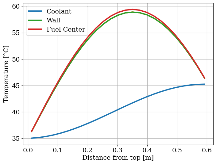
Here we will draw the temperature distribution along the channel (z-axis) of the coolant, the cladding and the fuel:

plt.figure()
plt.plot(C.centers, state[C.name]["T_cool"], label="Coolant")
plt.plot(C.centers, state[F.name]["T_wall_right"])
plt.plot(C.centers, state[F.name]["T_wall_left"], label="Wall")
plt.plot(
    C.centers,
    state[F.name]["T"].reshape(F.shape)[:, clad_N + int((fuel_N - 1) / 2)],
    label="Fuel Center",
)
plt.xlabel("Distance from top [m]")
plt.ylabel(r"Temperature [$\degree$C]")
plt.legend()
plt.grid()
plt.show()

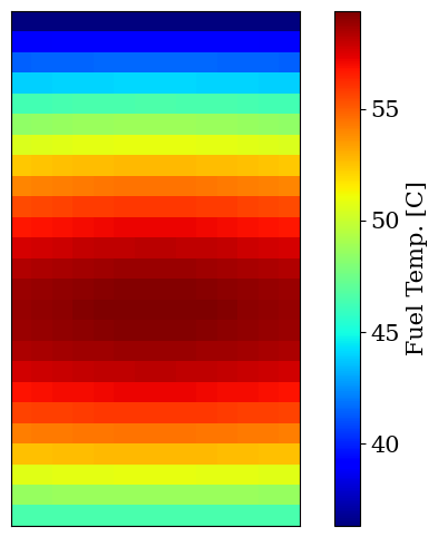
And here we will draw a color map of the temperature distribution of the fuel along the channel:

plt.figure(figsize=(8, 6))
ax = plt.imshow(state[F.name]["T"].reshape(F.shape), cmap="jet")
plt.colorbar(ax, label="Fuel Temp. [C]")
plt.xticks([])
plt.yticks([])
plt.show()